Forecasting Profits Direction in a Dataset of CAC40 Trades
Our dataset consists of many possible trades generated by several different strategies and our main purpose is to identify the most useful features in order to detect the trades with positive gain and therefore the winning strategies.
After having imported the data, we are going to clean in it up and to reformat them. Each record of the dataframe is a single transaction which consists of three trades. One trade to open the position and two trades to close it. A transaction can only be closed by taking a profit or by hitting a stop loss. For the moment we don’t need to consider the full dataset, we assume that the trades of the past 6 months are sufficient to have an accurate forecasting of the actual day.
# import data
dd = read.table("mytable.txt", header=T);
dd$dstart=as.Date(dd$dstart);
# get the trades of the past 6 months
tf=0.5; woy_test = as.Date("2020-09-18");
data = subset(dd, (dstart >= (woy_test-7)-trunc(365*tf)) & (dstart <= (woy_test-7)));
The number and type of features which are present in the dataframe depend of the trading strategies which are considered. In our case we have some general fields like the date of the main trade (i.e. dstart) with its entry time (i.e. hour), its direction (i.e. sign) and the expected number of points to hit a profit or a stop loss (i.e. tp_pts and sl_pts) which specifies all the required fields to execute a transaction. Then there are some fields about the result of the transaction, like the final pnl (i.e. pnl_simu) and how long the open position was kept before getting closed (i.e. lifetime).
All the other fields are additional information which are specific to the strategy which has generated the transaction. Actually most of them are the true features which we needs to exploit in order to forecast the pnl of the transaction. For example, pnl_day is the average pnl per day that the given strategy has generated in the past. While pf is the average profit factor up today. The last three columns (i.e. pnl_simu, mtm_dist_simu, lifetime) are the output of the tansaction so they cannot be part of the feature set for training.
> str(data)
'data.frame': 29860 obs. of 27 variables:
$ dstart : Date, format: "2020-03-16" "2020-03-16" ...
$ dend : Factor w/ 328 levels "2014-06-27","2014-07-04",..: 300 300 300 300 300 300 300 300 300 300 ...
$ woy : int 11 11 11 11 11 11 11 11 11 11 ...
$ yb : int 2 2 2 2 2 2 2 2 2 2 ...
$ max_pwrong_max : num 0.1 0.1 0.1 0.1 0.1 0.1 0.1 0.1 0.1 0.1 ...
$ min_avg_pnl_day: int 2 2 2 3 3 3 4 4 4 5 ...
$ dow : int 2 3 3 2 3 3 2 3 3 2 ...
$ hour : Factor w/ 32 levels "09:00:00","09:15:00",..: 6 1 4 6 1 4 6 1 4 6 ...
$ sign : int -1 1 -1 -1 1 -1 -1 1 -1 -1 ...
$ tp_pts : int 32 13 37 32 13 37 32 13 37 32 ...
$ sl_pts : int 23 8 12 23 8 12 23 8 12 23 ...
$ pnl : num 204 77.6 175 204 77.6 175 204 77.6 175 204 ...
$ pf : num 9.79 10.7 5.99 9.79 10.7 5.99 9.79 10.7 5.99 9.79 ...
$ ctr_tp : int 9 7 6 9 7 6 9 7 6 9 ...
$ ctr_sl : int 1 1 3 1 1 3 1 1 3 1 ...
$ ctr_tot : int 10 8 9 10 8 9 10 8 9 10 ...
$ pnl_day : num 20.4 9.7 19.4 20.4 9.7 19.4 20.4 9.7 19.4 20.4 ...
$ pwrong_max : num 0.0839 0.0403 0.0814 0.0839 0.0403 0.0814 0.0839 0.0403 0.0814 0.0839 ...
$ pwrong_max_h : num 0.905 0.753 0.898 0.905 0.753 0.898 0.905 0.753 0.898 0.905 ...
$ pwrong_max_n1 : num 1.9 1.92 1.91 1.9 1.92 1.91 1.9 1.92 1.91 1.9 ...
$ pwrong_max_n2 : num 1.64 1.7 1.67 1.64 1.7 1.67 1.64 1.7 1.67 1.64 ...
$ pwrong_max_n3 : num 0.899 1.05 0.974 0.899 1.05 0.974 0.899 1.05 0.974 0.899 ...
$ pwrong_max_n4 : num 0.331 0.474 0.396 0.331 0.474 0.396 0.331 0.474 0.396 0.331 ...
$ ccl_area : int 12 25 6 12 25 6 12 25 6 12 ...
$ pnl_simu : num 32 13 -12.5 32 13 -12.5 32 13 -12.5 32 ...
$ mtm_dist_simu : num 18 17 0 18 17 0 18 17 0 18 ...
$ lifetime : int 6 4 1 6 4 1 6 4 1 6 ...
Since we are interested only to detect the gaining trades a bare classification is sufficient so we can add a class field to our dataframe and to reformat some of the fields in order to have a dataset which is consistent with the classification process.
# clean up
data = data[-which(data$pnl_simu == 0),];
# remove na's if you have them
if(anyNA(data)) data = na.omit(data);
# add class
data$class = sign(data$pnl_simu);
data$class = factor(data$class, labels=c("N", "P"));
# reformat
data$hour = as.numeric(data$hour);
data$dstart = as.numeric(data$dstart);
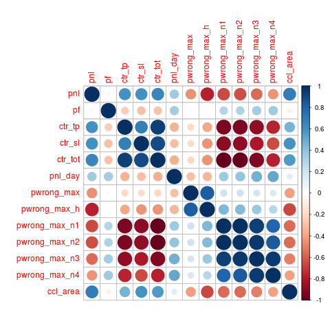
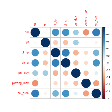
It is also interesting to check if some predictors used for forecasting are strongly correlated because, of course, they don’t bring any additional information for learning and so they can be safely removed. In particular, we can see that all the pwrong_max_nx variables and ctr_tot are strongly correlated so we removed them.
# correlation analysis
library(corrplot)
cm = cor(data[, 12:24]); corrplot(cm);
cm = cor(data[, c(12:15, 17:18, 24)]); corrplot(cm);
feat = c(12:15, 17:18, 24);
We will start considering a random forest model. Data is partitioned in two sets, one for training and one for testing. Training is done by the caret package. Many options can be selected, we opted for repeated cross validation in order to have a robust fitting and ROC as key metric for the loss function.
# training RF model
library(caret)
library(parallel)
library(doParallel)
# enable parallel computing
myCluster = makeCluster(detectCores()-1);
registerDoParallel(myCluster);
# features selection
fset = c(c("dstart", "dow", "hour"), names(data)[feat], "class");
# splitting training and testing dataset
set.seed(567);
inTrain = createDataPartition(y = data$class, p = .75, list = FALSE);
training = data[inTrain, fset];
testing = data[-inTrain, fset];
# training
set.seed(567);
ctrl = trainControl(method = "repeatedcv", repeats = 3, classProbs = TRUE, summaryFunction = twoClassSummary);
rfFit = caret::train(class ~ ., data = training, method = "rf", preProc = c("center", "scale"), tuneLength = 5, trControl = ctrl, metric = "ROC", allowParallel=T);
# training result
rfFit
Random Forest
48974 samples
10 predictors
2 classes: 'N', 'P'
Pre-processing: centered (10), scaled (10)
Resampling: Cross-Validated (10 fold, repeated 3 times)
Summary of sample sizes: 44077, 44076, 44076, 44076, 44076, 44077, ...
Resampling results across tuning parameters:
mtry ROC Sens Spec
2 0.9999080 0.9951705 0.9954507
4 0.9999126 0.9953134 0.9955807
6 0.9999115 0.9954277 0.9955677
8 0.9999087 0.9955991 0.9956977
10 0.9999016 0.9956848 0.9954767
ROC was used to select the optimal model using the largest value.
The final value used for the model was mtry = 4.
Learning by cross-validation results on an astonishing ROC of 0.999 for mtry=4 and sens/spec of 0.995. We can test our model on an independent dataset in order to validate the out-of-sample ROC/sens/spec metrics.
# ROC graph
library(pROC)
# prediction
rfProbs = predict(rfFit, newdata = testing[, -ncol(testing)], type = "prob");
rfClasses = predict(rfFit, newdata = testing[, -ncol(testing)]);
# testing CM and ROC
CM = caret::confusionMatrix(rfClasses, testing$class, positive="P");
ROC = roc(response = testing$class, predictor = rfProbs[,2], levels = rev(levels(testing$class)));
plot(ROC, lwd=2, col="red"); auc(ROC);
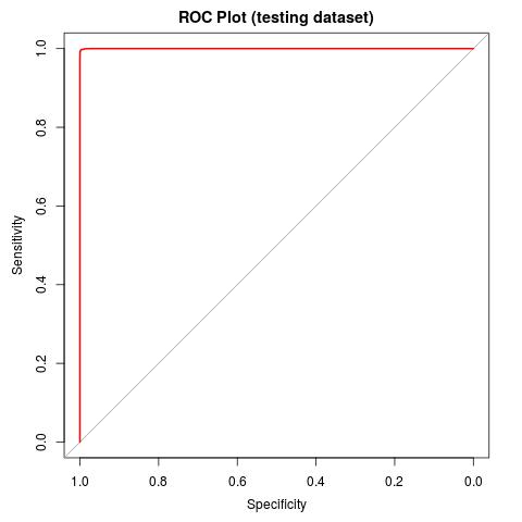
The results of testing are extremely similar to the metrics of the training, so confronting us on the good quality of model. Even the ROC plot looks so good that it is almost incredible. Unfortunately, as it is often in life, such result is too good to be true ! It will be sufficient to apply our model to the predictions of the actual days in order to discover that accuracy, sensitivity and any other possible metric are in fact much worse than the predicted ones. We are in a typical case of overfitting!
# testing results: CM
Confusion Matrix and Statistics
Reference
Prediction N P
N 3405 13
P 18 3214
Accuracy : 0.9967
95% CI : (0.9957, 0.9975)
No Information Rate : 0.5228
P-Value [Acc > NIR] : < 2e-16
Kappa : 0.9934
Mcnemar's Test P-Value : 0.07688
Sensitivity : 0.9977
Specificity : 0.9956
Pos Pred Value : 0.9960
Neg Pred Value : 0.9974
Prevalence : 0.5228
Detection Rate : 0.5216
Detection Prevalence : 0.5236
Balanced Accuracy : 0.9966
'Positive' Class : P
The verif dataset consists of the trades of five days of the actual week. It is cleaned it up and formatted, like we already did for training/testing datasets, and duplicated trades with same day/hour are removed. Then rfFit model is applied for forecasting, CM and ROC are computed.
# create a dataset for verification
verif = subset(dd, (dstart >= woy_test-4) & (dstart <= woy_test));
verif = verif[-which(verif$pnl_simu == 0),];
if(anyNA(verif)) verif = na.omit(verif);
verif$class = sign(verif$pnl_simu);
verif$class = factor(verif$class, labels=c("N", "P"));
verif$hour = as.numeric(verif$hour);
verif$dstart = as.numeric(verif$dstart);
verif_split=group_split(verif %>% group_by(dstart, dow, hour));
verif_unique = ldply(lapply(verif_split, function(x) as.data.frame(x)[1,]), rbind);
verif_pnl_simu = data.frame(pnl_simu=verif_unique$pnl_simu); rownames(verif_pnl_simu) = rownames(verif_unique);
verif = verif_unique[, fset];
# forecasting, CM and ROC
rfProbs = predict(rfFit, newdata = verif[, -ncol(verif)], type = "prob");
rfClasses = predict(rfFit, newdata = verif[, -ncol(verif)]);
CM = caret::confusionMatrix(rfClasses, verif$class, positive="P");
ROC = roc(response = verif$class, predictor = rfProbs[,2], levels = rev(levels(verif$class)));
plot(ROC, lwd=2, col="red", main="ROC Plot (verif dataset)"); grid(); auc(ROC);
# verif results: CM
Confusion Matrix and Statistics
Reference
Prediction N P
N 7 7
P 5 7
Accuracy : 0.5385
95% CI : (0.3337, 0.7341)
No Information Rate : 0.5385
P-Value [Acc > NIR] : 0.5796
Kappa : 0.0824
Mcnemar's Test P-Value : 0.7728
Sensitivity : 0.5000
Specificity : 0.5833
Pos Pred Value : 0.5833
Neg Pred Value : 0.5000
Prevalence : 0.5385
Detection Rate : 0.2692
Detection Prevalence : 0.4615
Balanced Accuracy : 0.5417
'Positive' Class : P
auc(ROC);
Area under the curve: 0.6815
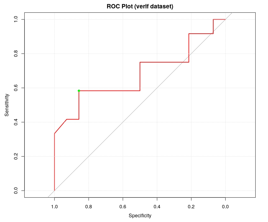
Unfortunately the predictions of the rfFit model to the verif dataset are not very good, the ROC plot has an AUC of 0.68 which basically means that the model has limited capacity to distinguish between positive class and negative class. In fact, it is only marginally better than a random discriminator. Therefore it is not possible to predict in a safe way whether a new transaction is going to produce a profit or a loss.
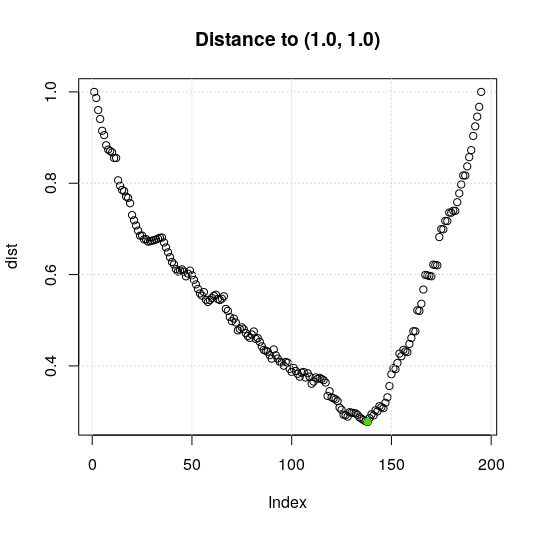
Still, it is possible to gain some marginal improvement of such classification by changing the probability threshold used to discriminate between P and N classes. Instead of adopting the default value of 0.5, we can look for the optimal value which will result on an higher accuracy and sensitivity/specificity. Such optimal value can be computed by detecting on the ROC plot the nearest point to the corner (1.0, 1.0).
# computing optimal threshold on verif
dist = (ROC$sensitivities-1)^2+(ROC$specificities-1)^2;
id = which.min(dist); opt_threshold = ROC$threshold[id];
plot(dist, main="Distance to (1.0, 1.0)"); grid(); points(id, dist[id], col="green", pch=16);
CM = caret::confusionMatrix(table(rfProbs[, "P"] >= 0.354, verif$class == "P"), positive="TRUE")
By computing the point at minimal distance, green point in the following figure, we get an optimal threshold of 0.354. The new CM is the following one where we can see the performance metrics are quite improved.
# verif results: CM
Confusion Matrix and Statistics
FALSE TRUE
FALSE 7 3
TRUE 5 11
Accuracy : 0.6923
95% CI : (0.4821, 0.8567)
No Information Rate : 0.5385
P-Value [Acc > NIR] : 0.08294
Kappa : 0.3735
Mcnemar's Test P-Value : 0.72367
Sensitivity : 0.7857
Specificity : 0.5833
Pos Pred Value : 0.6875
Neg Pred Value : 0.7000
Prevalence : 0.5385
Detection Rate : 0.4231
Detection Prevalence : 0.6154
Balanced Accuracy : 0.6845
'Positive' Class : TRUE
auc(ROC);
Area under the curve: 0.5609
It is interesting to compare the expected pnl from adopting the two possible thresholds of 0.5 and 0.354. As we expected the differences are important because higher values of sensitivity/specificity resulted on an overall positive pnl for the week when the default threshold wouldn’t have produced any.
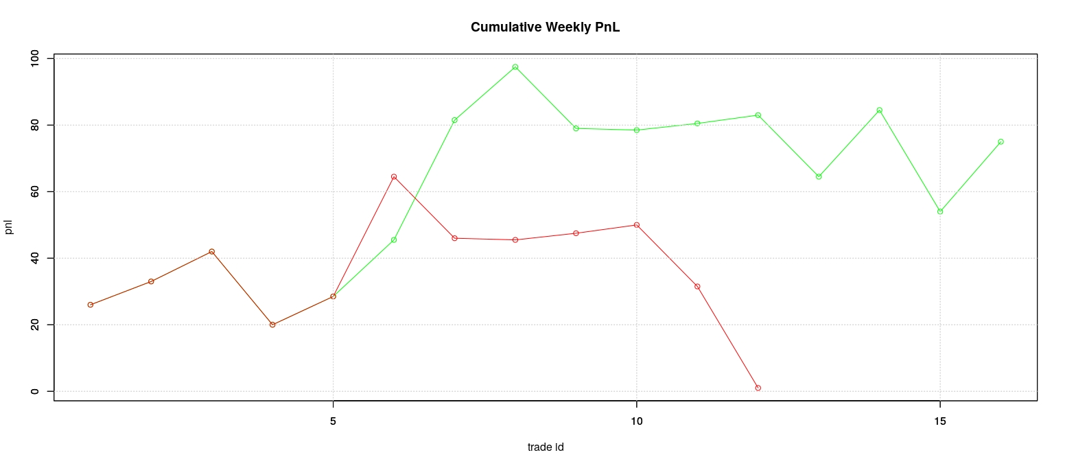
Now, the good choice of the threshold seems to be essential to select a winning strategy. Unfortunately, the approach we adopted to compute the optimal threshold cannot be applied in the practice because we exploited the posterior knowledge of trade results in our computation. However, the intuition that the choice of a good threshold can be sufficient to provide a positive pnl even when the forecasting model has somehow limited forecasting capabilities like in our case, it is an interesting fact.