Forecasting Profits Direction: Logistic Model
In the previous posts we developed a random forest model and walk-forward validation approach to forecast the direction of trades in a CAC40 dataset. Here we investigate the adoption of a logistic model instead of random forests. Since we still adopt a walk-forward validation, we will actually adopt an ensemble of logistic models, one for each of the walk-forward splitting.
Logistic modeling is quite common in binary classification problems, it is based on simple math which extends the linear regression approach, it has a nice bayesian interpretation and it can be seen as a single-layer perceptron so a first step in the world of neural networks and deep learning. Overall, it is a model that is worth testing!
# splitting training and testing dataset
part = createDataPartitionWT(y = data$dstart, p = .75);
# training ensemble logistic models
glmFit = list();
for(k in 1:part$num) {
training = data[part$train[[k]], fset];
set.seed(567);
ctrl = trainControl(method = "cv", number = 5, classProbs = TRUE, savePredictions = "all", allowParallel=T);
glmFit[[k]] = caret::train(class ~ ., data = training, method = "glm", family = "binomial", preProc = c("center", "scale"), trControl = ctrl);
}
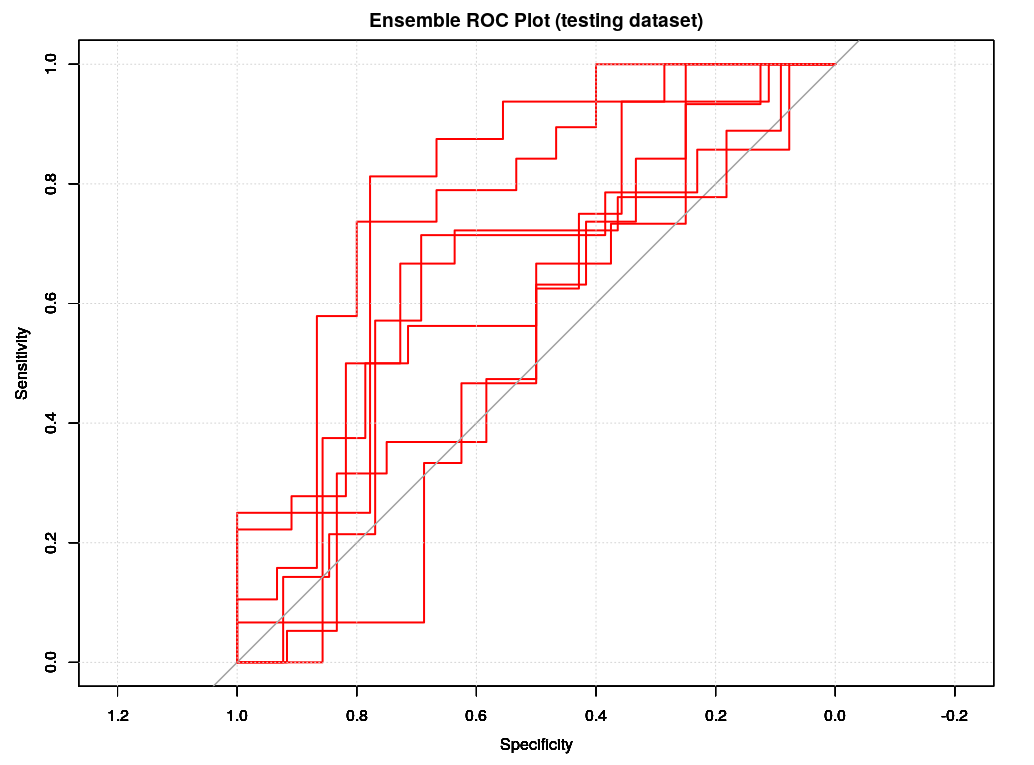
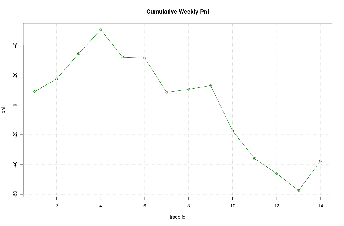
Following the training, we can check the ROC plots for both the testing and verif datasets. The results are not surprising, sensitivity and specificity are much worse in the verification datasets. However, what is somehow surprising, is that comparing the ROC of the verif datasets with previous random forest model we will see that logistic classification seems to be worse and this is also confirmed by both the CM and the expected cumulative pnl for the coming week.
# verif results: CM
Confusion Matrix and Statistics
Reference
Prediction N P
N 5 7
P 7 7
Accuracy : 0.4615
95% CI : (0.2659, 0.6663)
No Information Rate : 0.5385
P-Value [Acc > NIR] : 0.8373
Kappa : -0.0833
Mcnemar's Test P-Value : 1.0000
Sensitivity : 0.5000
Specificity : 0.4167
Pos Pred Value : 0.5000
Neg Pred Value : 0.4167
Prevalence : 0.5385
Detection Rate : 0.2692
Detection Prevalence : 0.5385
Balanced Accuracy : 0.4583
'Positive' Class : P
auc(ROC);
Area under the curve: 0.494
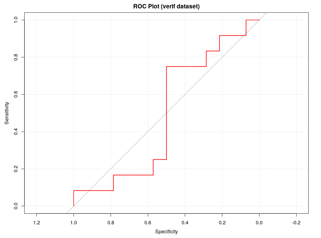
Overall, the logistic model seems to be much less selective that the random forest one, we have more trades 14 instead of 6 but unfortunately the accuracy of forecasting is not improved, so resulting on a much worse expected pnl (around -40 instead of +7).
A nice thing about logistic model is that they support and easy interpretation of the forecasting result. It is sufficient to check the fitted models to identify the features which contributes most to the classification process. For example checking the seven logistic models by the summary() function we found that only three features are really important in the classification: ctr_tp, ctr_sl and ccl_area.
summary(glmFit[[7]]);
Deviance Residuals:
Min 1Q Median 3Q Max
-1.8650 -1.0848 -0.8134 1.1854 1.9316
Coefficients:
Estimate Std. Error z value Pr(>|z|)
(Intercept) -0.09850 0.08912 -1.105 0.26905
dstart -0.06235 0.09139 -0.682 0.49506
dow 0.10158 0.10002 1.016 0.30979
hour -0.05234 0.09246 -0.566 0.57130
pnl -0.38413 0.24534 -1.566 0.11741
pf -0.12350 0.11852 -1.042 0.29742
ctr_tp 0.68536 0.17379 3.944 8.03e-05 ***
ctr_sl -0.54886 0.18478 -2.970 0.00298 **
pnl_day 0.21208 0.17444 1.216 0.22405
pwrong_max 0.02765 0.10431 0.265 0.79092
ccl_area 0.47819 0.16730 2.858 0.00426 **
---
Signif. codes: 0 ‘***’ 0.001 ‘**’ 0.01 ‘*’ 0.05 ‘.’ 0.1 ‘ ’ 1
( Dispersion parameter for binomial family taken to be 1)
Null deviance: 745.86 on 538 degrees of freedom
Residual deviance: 712.07 on 528 degrees of freedom
AIC: 734.07
Number of Fisher Scoring iterations: 4
car::Anova(glmFit[[7]]$finalModel);
Analysis of Deviance Table (Type II tests)
Response: .outcome
LR Chisq Df Pr(>Chisq)
dstart 0.4660 1 0.494842
dow 1.0347 1 0.309051
hour 0.3208 1 0.571135
pnl 2.4643 1 0.116458
pf 1.1863 1 0.276073
ctr_tp 16.8027 1 4.147e-05 ***
ctr_sl 9.3435 1 0.002238 **
pnl_day 1.4855 1 0.222909
pwrong_max 0.0702 1 0.791025
ccl_area 8.6183 1 0.003328 **
---
Signif. codes: 0 ‘***’ 0.001 ‘**’ 0.01 ‘*’ 0.05 ‘.’ 0.1 ‘ ’ 1
We could push the analysis a step further by retraining a logistic model considering only such “important” features and, then, by analyzing their crossed behaviors.
# fit a reduced set of features
training = data[part$train[[7]], fset];
fit = glm(class ~ ., data = training[c("ctr_tp", "ctr_sl", "ccl_area", "class")], family = "binomial");
# training results
summary(fit)
Call:
glm(formula = class ~ ., family = "binomial", data = training[c(6, 7, 10, 11)])
Deviance Residuals:
Min 1Q Median 3Q Max
-1.8616 -1.0799 -0.8389 1.2237 1.7239
Coefficients:
Estimate Std. Error z value Pr(>|z|)
(Intercept) -0.6088330 0.1720067 -3.540 0.000401 ***
ctr_tp 0.0623430 0.0146327 4.261 2.04e-05 ***
ctr_sl -0.0923482 0.0232163 -3.978 6.96e-05 ***
ccl_area 0.0017915 0.0006155 2.911 0.003606 **
---
Signif. codes: 0 ‘***’ 0.001 ‘**’ 0.01 ‘*’ 0.05 ‘.’ 0.1 ‘ ’ 1
(Dispersion parameter for binomial family taken to be 1)
Null deviance: 745.86 on 538 degrees of freedom
Residual deviance: 716.97 on 535 degrees of freedom
AIC: 724.97
Number of Fisher Scoring iterations: 4
# plot features behavior
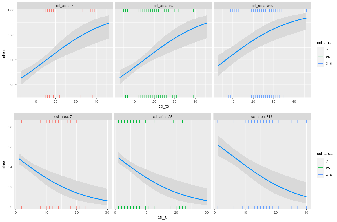
visreg(fit, scale="response", gg=T, xvar="ctr_tp", by="ccl_area", rag=2);
visreg(fit, scale="response", gg=T, xvar="ctr_sl", by="ccl_area", rag=2);
# plot ROC
df = data.frame(class = training$class, prob = fit$fitted.values);
ggplot(df, aes(d = class, m = prob)) + geom_roc() + style_roc() + labs(title="Ensemble ROC Plot (testing dataset)");
The probability of having a profit increase by increasing ctr_tp and decreasing ctr_sl as it was expected. More interesting, higher values of ccl_area contribute to a positive pnl but not in a linear way, it looks like only values greater than 100 are relevant.
The ROC plots of the seven models of the ensemble have similar shapes, and this is quite good news, it means that the overall behaviour of the logistic model with a reduced set of features is quite stable despite the walk-forward splitting. A threshold around 0.6 seems to be a common optimal point.
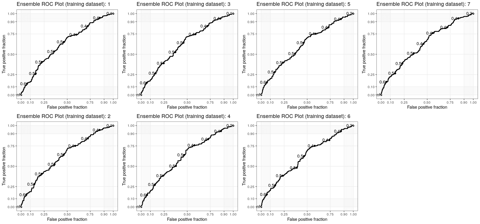
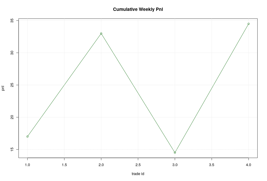
The adoption of such optimal threshold will result in an improved estimated pnl.
