Forecasting Profits Direction: Walk-Forward Validation
In a previous post we developed a random forest model to forecast the direction of trades in a CAC40 dataset. Despite the fact that the training accuracy was extremely high, the forecasting metrics resulted quite poor. Generally speaking, such kind of discrepancy is a clear evidence of overfitting in the learning process: the model is not able to generalize because it fitted too much with the training data.
Of course, overfitting can be reduced by constraining the learning process and therefore trading an increase in its generalization capabilities for reduced training metrics - and this can be done in our case, for example, by constraining the number of generated trees in the random forest. However, this is not going to improve the forecasting metrics anyway. In addition, there is another source of overfitting in our specific case. A sequence of trades, day after day or week after week, can be seen as a time series when they come from the same strategy i.e. the trades are not statistically independent. So, applying a cross validation approach like we did in order to have a robust learning process, it will inevitably result on a misleading good learning metrics because we implicitly peaked some data into the future. Somehow we looked ahead by adopting the cross validation.
A common approach to avoid such pitfall in time series training is to validate the training by a walk-forward splitting. The idea is simple, first we need to order our trades dataset by a time tag (which by the way is already present having day/hour fields) then we can split it according to a defined proportion and to apply our training /validation process in a sequence of train/test subsets like reported in the following picture. Eventually, a rolling windows can be considered if we don’t want to have an increasing training set.

The following procedure createDataPartitionWT() takes a vector of time tags y and it returns a set of train and test sets according to the walk-through splitting approach.
createDataPartitionWT = function(y, p=0.75) {
# save original data tag sequence
dt = data.frame(id=1:length(y), data=y);
# train/test sets size
ns = length(unique(y));
ns_train = max(1, trunc(ns*p)); ns_test = ns-ns_train;
if (ns_test < 1) stop("Error, not enough unique time tags to split!\n");
# order the time tags and partition it into ns sets
dt_ord = dt[order(dt$data), ]; dt_ord$slot=0;
dt_un = unique(y);
for( k in 1:ns) { idx = which(dt_ord$data == dt_un[k]); dt_ord$slot[idx] = k; }
# create ns_test train and test sets by rolling window
train=list(); test=list();
for(k in 1:ns_test) {
idx = which((dt_ord$slot <= ns_train+k-1) & (dt_ord$slot >= k));
train[[k]] = dt_ord$id[idx];
idx = which(dt_ord$slot == ns_train+k);
test[[k]] = dt_ord$id[idx];
}
return(list(num=ns_test, train=train, test=test));
}
Compared to our previous post where we adopted a bare rf model, now we need to use a set of rf models because we have a set of train/test set instead of a single one. Therefore, we are going to adopt what is called an ensemble method in machine learning: multiple models are trained on the same initial dataset at first, then forecasting is based on combination of their multiple predictions. In our case, all the adopted models are rf and, since we are interested to the classification of trades, forecasted results can be combined either by majority of results or by averaging their probabilities.
# splitting training and testing dataset
part = createDataPartitionWT(y = data$dstart, p = .75);
# training ensemble rf models
rfFit = list();
for(k in 1:part$num) {
training = data[part$train[[k]], fset];
set.seed(567);
ctrl = trainControl(method = "oob", classProbs = TRUE, savePredictions = "all");
rfFit[[k]] = caret::train(class ~ ., data = training, method = "rf", preProc = c("center", "scale"), tuneLength = 5, maxnodes=50, trControl = ctrl, allowParallel=T);
}
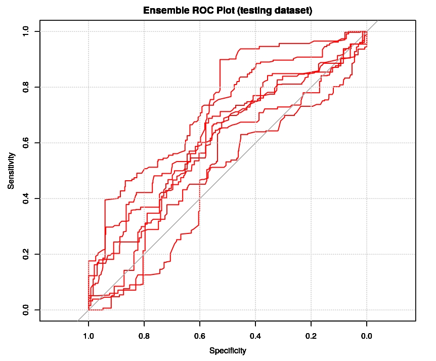
The cumulative plot ROC shows us that the classification is far from be perfect, as instead we wrongly supposed to be in the original post. This is obviously not a good news but it showed us that overfitting was a true issue in the previous case and the real accuracy was well lower than 0.9967. It is also interesting to know that it is possible to have an estimation of the ROC of the ensemble classifier simply by computing the convex hull of such cumulative plot ROC in the case of a binary classifier, yet this is only a conservative estimation (see the paper from M. Barreno). In addition, an estimation of the likelihoods of the two forecasted classes can be obtained by the analysis of the ROC shape (see the paper from C. Marzaban).

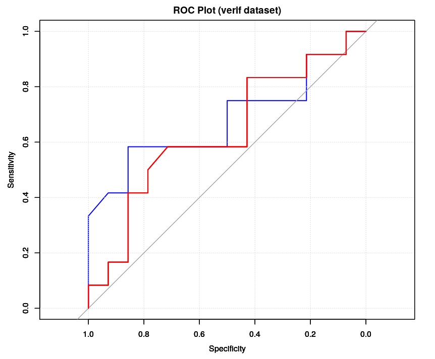
Finally, we can asses the performance of this new model on the verif dataset and to check both its CM nd ROC plot (red color, blue color is the previous one). Unfortunately, the results are extremely similar to what we get in the previous post, no major improvement in AUC neither in sensitivity or specificity.
# forecasting based on majority
# -------------------------------------------------------------------------------------------
rfProbs = matrix(, nrow = dim(verif)[1], ncol = part$num)
for(k in 1:part$num) {
rfProbs[,k] = predict(rfFit[[k]], newdata = verif[, -ncol(verif)], type = "prob")[,2];
}
# classification by majority - standard threshold
rfClasses = rep("N", dim(verif)[1]);
rfClasses[which(rowMeans(rfProbs) > 0.5)] = "P";
rfClasses = factor(rfClasses, levels=c("N", "P"), labels=c("N", "P"));
CM = caret::confusionMatrix(rfClasses, verif$class, positive="P");
ROC = roc(response = verif$class, predictor = rowMeans(rfProbs), levels = rev(levels(verif$class)));
plot(ROC, lwd=2, col="red", main="ROC Plot (verif dataset)"); grid(); auc(ROC);
# verif results: CM
Confusion Matrix and Statistics
Reference
Prediction N P
N 10 10
P 2 4
Accuracy : 0.5385
95% CI : (0.3337, 0.7341)
No Information Rate : 0.5385
P-Value [Acc > NIR] : 0.57965
Kappa : 0.1136
Mcnemar's Test P-Value : 0.04331
Sensitivity : 0.2857
Specificity : 0.8333
Pos Pred Value : 0.6667
Neg Pred Value : 0.5000
Prevalence : 0.5385
Detection Rate : 0.1538
Detection Prevalence : 0.2308
Balanced Accuracy : 0.5595
'Positive' Class : P
auc(ROC);
Area under the curve: 0.6339

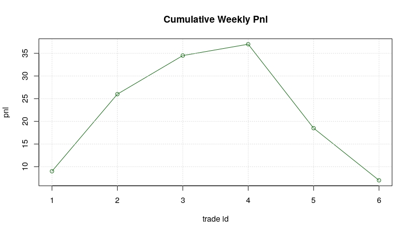
If we compute the expected cumulative pnl for the coming week we will get 7 CAC40 points which is somehow in the middle between what we got in the previous post (1 CAC40 point for the standard threshold of 0.5 and 75 CAC40 point for the optimal threshold of 0.354) but still far from the optimal value. So, a little better result nut nothing special!
